An Intro To Observational Studies
Observational, sometimes called retrospective, studies are an interesting concept and have many applications in my opinion. You can think of the goal of these studies as being to reverse engineer a statistical experiment as best as possible. Since most real life (observational) data was not set up in some sort of randomized design, we need a way to reduce bias and put control/treatment individuals on equal footing before estimating any sort of causal effects. One technique of doing this is called Matching.
Matching
Matching attempts to “balance” the distribution of covariates between control/treatment individuals. To do this, we first need some sort of distance metric to use between individuals, even if this is a highly dimensional problem. Some common ones are:
- Exact: only match individuals that have the same exact covariate values (useful if binary).
- Propensity score: absolute or linear difference in propensity scores, which is the conditional probabilty of an individual being a treatment given its covariates.
- Euclidean: sum of the normalized distanced for each covariate.
- Mahalanobis: euclidean distance adjusting for covariance in the data.
- Generalized Mahalanobis: a generalized version of the Mahalanobis distance to weight covariates by their importance to producing balance.
Using a caliper we can cap how large these distances can be for each covariate. As we become more stringent with the caliper, we throw more individuals out from consideration from each group, which you will see shortly.
Once we have distances between all individuals, we just need to match! There are a few different ways to do so:
- Nearest neighbor: for a treatment individual, find the closest control (minimize the distance). If there’s a tie, pick randomly.
- Optimal: finds the matching solution that minimizes overal distance. Could allow for one-to-many, where several weighted controls are matched to one treatment (or vice versa).
- GenMatch: a genetic algorithm that attempts to find the Mahalanobis weights that produce the best balance. Again one-to-many is possible.
Example
This example is for those of you who pay attention to the european soccer transfer news (ok ok gossip) like me. I discovered a really unique and extensive soccer data set, developed mainly by Hugo Mathien. I’ve been tinkering with it for a while and then one day I came up with a question I thought was worth investigating: When a player transfers to another team, how can you tell if he actually improved / performed better? The only way to properly test this would be to give him the exact same teammates, opponents, and game conditions for some amount of time, say a season or two, and then see if he scores more goals, gets more assists, makes more tackles, etc. But we don’t live in a world where this is possible, and that’s where an observational study comes in. What if I match games where the treatment is the club the player is representing? Obviously I would want to control for covariates like the overall skill / form of each team in the game, at what point in the season is the game, home or away status, weather, and maybe even betting odds. I believe doing so would allow us to better say if a player really got better after switching teams.
For this post, we’ll look at Gareth Bale. Specifically, we’ll look at his games playing for Tottenham and Real Madrid. We’ll try to find ones that look similar based on the attributes I mentioned above and then we’ll see if there’s a significant difference between his goals per game ratio for each club. See the Notes section at the bottom of this post for additional player and team IDs.
Data Background
As I mentioned, the data I’m using is a small sqlite database I found on
Kaggle here. The game
(Match) data spans from the 2008/2009 to 2015/2016 seasons. It only
contains the league games from 11 european countries, so no
Champions’/Europa League games are included. There’s also a ton of
betting odds for each game.
The data is just over 300MB and can be read into R like so:
    # Setting up environment

    library(RSQLite)
    library(dplyr)
    library(XML)
    library(lubridate)
    library(data.table)
    library(car)
    library(Matching)

    # Data Set

    db <- dbConnect(SQLite(), dbname="~/Documents/Kaggle/Soccer_Data/database.sqlite")
    dbListTables(db)
## [1] "Country" "League" "Match"
## [4] "Player" "Player_Attributes" "Team"
## [7] "Team_Attributes" "sqlite_sequence"
Data Prep
The function below helps to aggregate the data for use in our observational study. Some important things it does:
- Get the games our player of interest started in for each club.
- Create the treatment variable (1 if second team, 0 if first team) and parse some XML to get the player’s goals and assists per game.
- Find all player’s most recent overall rating from EA’s FIFA video game. EA updates these so I select the closest rating based on dates leading up to or on the date of the game. Get an average team rating for each team.
- Return a
data.frameand table with some relevant statistics.
    get_data <- function(pid,       #player ID (e.g. Gareth Bale's player ID)
                         team1id,   #First Team's ID (e.g. Tottenham's Team ID)
                         team2id,   #Second Team's ID (e.g. Real Madrid's Team ID)
                         con)       #Database connection object (e.g. db)
      {

      #treatment games are coming from the team the player moved to
      trt <- team2id

      #getting data sources
      matches <- data.frame(dbGetQuery(con,"SELECT * FROM Match"))
      players <- data.frame(dbGetQuery(con,"SELECT * FROM Player"))
      teams <- data.frame(dbGetQuery(con,"SELECT * FROM Team"))
      player_atts <- data.frame(dbGetQuery(con,"SELECT * FROM Player_Attributes"))

      #getting games involving these two teams and deleting player coordinate columns
      matches <- matches[matches$home_team_api_id %in% c(team1id,team2id) | matches$away_team_api_id %in% c(team1id,team2id),-c(12:55)]

      #keeping games where our player started
      final_matches <- matches[which(Vectorize(function(x) x %in% c(pid))(matches[,c(12:33)]),arr.ind=TRUE)[,1],]

      #we loop across each row of this data to do several things:
      #1) assign games as treatment/controls. It's not as easy as just assigning based on team, because what if teams are in the same league?
      #2) number of goals player scored each game. Found via parsing xml
      #3) nuber of assists player made each game. Found via parsing xml
      #4) creating a flag indicating whether the game was a home game

      treat <- vector()
      g <- vector()
      a <- vector()
      hf <- vector()

      for(i in 1:dim(final_matches)[1]) {

        r <- final_matches[i,]

        event_df <- xmlToDataFrame(r$goal)
        event_df <- event_df[!is.na(as.numeric(event_df$stats)),]
        g[i] <- sum(as.numeric(event_df$player1) == pid,na.rm=TRUE)
        a[i] <- sum(as.numeric(event_df$player2) == pid,na.rm=TRUE)

        if(r$home_team_api_id==trt & pid %in% r[,c(12:22)]) {
          treat[i] <- 1
        }
        else if(r$away_team_api_id==trt & pid %in% r[,c(23:33)]) {
          treat[i] <- 1
        }
        else { treat[i] <- 0 }

        if(pid %in% r[,c(12:22)]) {
          hf[i] <- 1
        }
        else {
          hf[i] <- 0
        }
      }

      final_matches$trt <- treat
      final_matches$player_goals <- g
      final_matches$player_assists <- a
      final_matches$home_flag <- hf

      #converting date columns for use in data.table
      final_matches$date <- ymd_hms(final_matches$date)
      player_atts$date <- ymd_hms(player_atts$date)
      player_atts <- player_atts[,c("player_api_id","date","overall_rating")]

      #this loop allows us to match a rating to each player in the starting 11, based on their fifa rating.
      #EA updates these so I select the closest rating based on dates leading up to or on game date, hence the use of the roll option
      nms <- names(final_matches[,c(12:33)])

      fm <- final_matches
      pa <- player_atts
      setDT(fm)
      setDT(pa)

      for(i in 1:length(nms)) {

        setkeyv(fm, c(nms[i], "date"))
        setkey(pa, "player_api_id", "date")[, closest_date:=date]
        test <- pa[fm, roll=Inf]

        fm[, nms[i] := test[, "overall_rating", with=FALSE], with=FALSE]
      }

      #calculate average home/away team ratings per game
      fm <- as.data.frame(fm)
      fm$home_rating_avg <- rowMeans(fm[,12:22], na.rm = TRUE)
      fm$away_rating_avg <- rowMeans(fm[,23:33], na.rm = TRUE)

      #table of stats
      t <- c(teams$team_long_name[teams$team_api_id==team1id],teams$team_long_name[teams$team_api_id==team2id])
      games <- c(length(which(fm$trt==0)),length(which(fm$trt==1)))
      goals <- c(sum(fm$player_goals[fm$trt==0]),sum(fm$player_goals[fm$trt==1]))
      assists <- c(sum(fm$player_assists[fm$trt==0]),sum(fm$player_assists[fm$trt==1]))

      tbl <- rbind(games,goals,assists)
      colnames(tbl) <- t
      return(list(data=fm,tbl=tbl))

    }
Let’s call this function. Again, see the Notes section at the bottom of this post for additional player and team IDs.
    bale <- get_data(pid = 31921,
                     team1id = 8586,
                     team2id = 8633,
                     con=db)

    bale$tbl
## Tottenham Hotspur Real Madrid CF
## games 128 75
## goals 25 29
## assists 13 17
We can see that Gareth has more goals as a madridista, even while playing less games. But could this be because he’s in an easier league or with better teammates? Let’s use Matching to find out.
Matching
Let’s look at Matching in a way I find intuitive: visually through multivariate plots. Since Matching “balances” covariates, we can think of the joint distributions of our control and treatment groups to become more overlapped the better the balance. So if I use the home and away teams’ average rating for each game, we see something like below. Can you guess where los clasicos are ;)?
    dataEllipse(bale$data$home_rating_avg, bale$data$away_rating_avg, as.factor(bale$data$trt), asp=1, levels=0.5, lwd=2, center.pch=16,
                xlab= "Home Team Avg. Rating", ylab= "Away Team Avg. Rating", xlim= c(65,87), ylim= c(65,87),
                col=c("blue","black"), main="Joint distribution of two variables (before matching)")
    legend(x="topleft", legend=c("Real Madrid", "Tottenham"), pch=c(2,1), col=c("black", "blue"))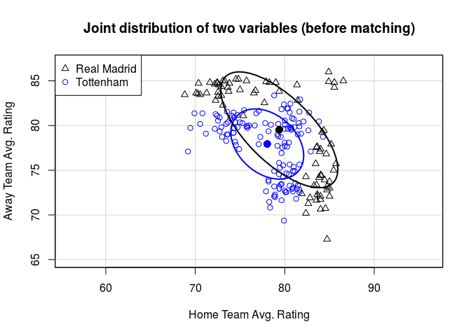
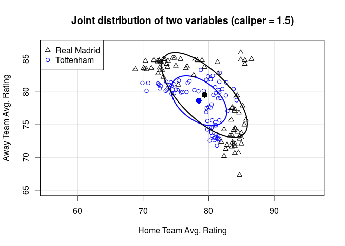
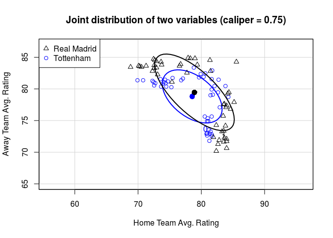
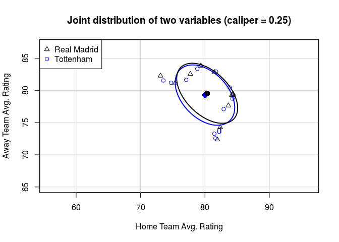
If we do a quick and dirty Matching and tighten our caliper, you can see that the distribtuions begin to overlap more. However we throw out more and more individual games while doing so. This is always the tradeoff with Matching.
    x <- cbind(bale$data$home_rating_avg , bale$data$away_rating_avg)  #covariates to match on
    tr <- bale$data$trt                                                #treatment variable
    y <- bale$data$player_goals                                        #response we're measuring

    cals <- c(1.5,0.75,0.25)                                           #calipers to loop over

    for(i in cals){

      m <- Match(Y=y,
                 Tr=tr,
                 X=x,
                 M=1,
                 replace = FALSE,
                 caliper=i,
                 ties=FALSE,
                 Weight=2)

      title <- paste0("Joint distribution of two variables (caliper = " , i, ")",sep="")

      dataEllipse(m$mdata$X[,1], m$mdata$X[,2], as.factor(m$mdata$Tr), asp=1, levels=0.5, lwd=2, center.pch=16,
                  xlab= "Home Team Avg. Rating", ylab= "Away Team Avg. Rating", xlim= c(65,87), ylim= c(65,87),
                  col=c("blue","black"), main=title)
      legend(x="topleft", legend=c("Real Madrid", "Tottenham"), pch=c(2,1), col=c("black", "blue"))

    }
Now let’s do a more technical Matching. I will match on the following covariates:
- stage = what number game in the league season it is
- B365H = Bet365 home win odds
- B365D = Bet365 draw odds
- B365A = Bet365 away win odds
- home_rating_avg: home team’s average EA FIFA rating
- away_rating_avg: away team’s average EA FIFA rating
In a perfect world where I had a bit more data, I would include a flag for whether the game is home or away, if it’s near another fixture such as a cup game, weather conditions, etc.
    x <- as.matrix(bale$data[,c(5,42:44,76:77)])   #covariates to match on
    tr <- bale$data$trt                            #treatment variable
    y <- bale$data$player_goals                    #response we're measuriong
    names(bale$data[,c(5,42:44,76:77)])
## [1] "stage" "B365H" "B365D" "B365A"
## [5] "home_rating_avg" "away_rating_avg"
See my comments below and the Matching package’s
documention
for more insight as to what these parameters are doing in this optimal
matching scenario:
    m <- Match(Y=y,
          Tr=tr,
          X=x,
          M=1, replace=TRUE,                           #one-to-one matching with replacement
          caliper=2.0,                                 #how large these distribution are allowed to span
          ties=TRUE,                                   #ties are allowed, weighted means are calculated if necessary
          Weight=2)                                    #Mahalanobis distance
It is always recommended to check the balance of your covariates using this function. I won’t print this function since it is reallllllly long, but basically you should at the minimum look to see if your variance ratio of treatments to controls got closer to 1 and your Kolmogorov-Smirnov tests are significant.
mb <- MatchBalance(tr ~ x, match.out = m, nboots = 1000)Results
length(m$index.treated)## [1] 58
length(m$index.control)## [1] 58
Our matching kept 58 games for each group, totalling to 116 games. What’s the difference in goals per game for Gareth’s matched Tottenham and Real Madrid games?
m$est## [,1]
## [1,] 0.2586207
Wow! So when controlling for “similar” games he played in for Tottenham and Real Madrid, we estimate that Gareth scores on average a quarter of a goal more per game as a madridista! But is this result statistically significant?
    CIs <- cbind(m$est - 1.96*m$se.standard , m$est + 1.96*m$se.standard)
    colnames(CIs) <- c("Lower 95 Conf. Level" , "Upper 95 Conf. Level")
    CIs
## Lower 95 Conf. Level Upper 95 Conf. Level
## [1,] 0.03671373 0.4805277
Using a 95% confidence interval, I would say yes!
Assumptions, Caveats, & Other Considerations
As I mentioned earlier, there are other covariates I could’ve used that
theoretically make sense and could potentially improve the balance. I
could’ve included a propensity score as a covariate or even matched
using GenMatch()’s genetic algorithm. It’s also important to note that
I’m pushing the boundaries when it comes to sample sizes in this
example. More games for each team would’ve been preferable.
In terms of the causal effect I estimated remember a couple things:
- This effect only applies to the games I matched on and not all the other games. By doing this we are obviously throwing away a lot of data.
- This method is simply a nonparameteric way of estimating a causal effect. “Without an experiment, natural experiment, a discontinuity, or some other strong design, no amount of econometric or statistical modeling can make the move from correlation to causation persuasive” - Jasjeet S. Sekhon.
Resources
I eventually figured out how to join player ratings using the closest date thanks to this post.
For more technical details on Matching and its implemenation in R
check out this
paper.
The kaggle discussion board was helpful in general, particularly on how to parse the XML game event data to get goals and assists by player.
Notes
I hope you find these tables useful for your own study!
    matches <- data.frame(dbGetQuery(db,"SELECT * FROM Match"))
    players <- data.frame(dbGetQuery(db,"SELECT * FROM Player"))
    teams <- data.frame(dbGetQuery(db,"SELECT * FROM Team"))
    player_atts <- data.frame(dbGetQuery(db,"SELECT * FROM Player_Attributes"))

    player_list <- c("Robin van Persie", "Gareth Bale","Luis Suarez","Diego Costa","Edinson Cavani",
                     "Cesc Fabregas","Robert Lewandowski","Gonzalo Higuain","Luka Modric",
                     "Alexis Sanchez","Mesut Oezil","Radamel Falcao","Zlatan Ibrahimovic",
                     "Sergio Aguero","Mario Goetze", "Eden Hazard","David Villa","Juan Mata",
                     "Edin Dzeko","Ezequiel Lavezzi","Fernando LLorente","Daniel Sturridge",
                     "Alessandro Matri","Carlos Tevez","David Silva"
    )
    p <- dplyr::filter(players, grepl(paste(player_list, collapse="|"), player_name))
    p[,c(2,3,5,6,7)]
## player_api_id player_name birthday height weight
## 1 41411 Alessandro Matri 1984-08-19 00:00:00 182.88 176
## 2 50047 Alexis Sanchez 1988-12-19 00:00:00 170.18 137
## 3 38817 Carlos Tevez 1984-02-05 00:00:00 172.72 157
## 4 30613 Cesc Fabregas 1987-05-04 00:00:00 175.26 163
## 5 51553 Daniel Sturridge 1989-09-01 00:00:00 187.96 168
## 6 37459 David Silva 1986-01-08 00:00:00 170.18 148
## 7 30909 David Villa 1981-12-03 00:00:00 175.26 152
## 8 19243 Diego Costa 1988-10-07 00:00:00 187.96 187
## 9 107417 Eden Hazard 1991-01-07 00:00:00 172.72 163
## 10 15403 Edin Dzeko 1986-03-17 00:00:00 193.04 185
## 11 49677 Edinson Cavani 1987-02-14 00:00:00 182.88 157
## 12 18925 Ezequiel Lavezzi 1985-05-03 00:00:00 172.72 165
## 13 31921 Gareth Bale 1989-07-16 00:00:00 182.88 163
## 14 25759 Gonzalo Higuain 1987-12-10 00:00:00 182.88 181
## 15 41468 Juan Mata 1988-04-28 00:00:00 170.18 139
## 16 40636 Luis Suarez 1987-01-24 00:00:00 182.88 187
## 17 31097 Luka Modric 1985-09-09 00:00:00 175.26 143
## 18 177714 Mario Goetze 1992-06-03 00:00:00 175.26 159
## 19 36378 Mesut Oezil 1988-10-15 00:00:00 182.88 168
## 20 22543 Radamel Falcao 1986-02-10 00:00:00 177.80 159
## 21 93447 Robert Lewandowski 1988-08-21 00:00:00 185.42 174
## 22 30843 Robin van Persie 1983-08-06 00:00:00 187.96 157
## 23 37412 Sergio Aguero 1988-06-02 00:00:00 172.72 163
## 24 35724 Zlatan Ibrahimovic 1981-10-03 00:00:00 195.58 209
    team_list <- c("Madrid","Valencia","Barcelona","Arsenal","Chelsea","Tottenham",
                   "Liverpool","Manchester","Napoli","Juventus","Milan","Inter","Cagliari",
                   "Paris","Lille","Monaco","Wolfsburg","Dortmund","Bayern Munich"
    )
    t <- dplyr::filter(teams, grepl(paste(team_list, collapse="|"), team_long_name))
    t[,c(2,4)]
## team_api_id team_long_name
## 1 10260 Manchester United
## 2 9825 Arsenal
## 3 8650 Liverpool
## 4 8456 Manchester City
## 5 8586 Tottenham Hotspur
## 6 8455 Chelsea
## 7 9829 AS Monaco
## 8 9847 Paris Saint-Germain
## 9 8639 LOSC Lille
## 10 9823 FC Bayern Munich
## 11 9789 Borussia Dortmund
## 12 8721 VfL Wolfsburg
## 13 8529 Cagliari
## 14 9885 Juventus
## 15 8564 Milan
## 16 9875 Napoli
## 17 8636 Inter
## 18 10267 Valencia CF
## 19 8633 Real Madrid CF
## 20 8634 FC Barcelona
## 21 9906 Atlético Madrid